Keynesian Theory of Income and Employment: Output and Employment 2020

Keynesian Theory of Income and Employment

• Keynesian theory of employment depends upon effective demand. Effective demand results in the output. Output creates income. Income provides employment. Since Keynes assumes all these four quantities, viz., effective demand (ED), output (Q), income (Y), and employment (N) equal to each other, he regards employment as a function of income.
• Effective demand is determined by two factors, the aggregate supply function and the aggregate demand function. The aggregate supply function depends on physical or technical conditions of production which do not change in the short-run.
• Since Keynes assumes the aggregate supply function to be stable, he concentrates his entire attention upon the aggregate demand function to fight depression and unemployment. Thus employment depends on aggregate demand which in turn is determined by consumption demand and investment demand.
• According to Keynes, employment can be increased by increasing consumption and/or investment. Consumption depends on income C(Y) and when income increases, consumption also increases but at a diminishing rate. In other words, as income rises, saving rises.
• Consumption can be increased by raising the propensity to consume in order to increase income and employment. But the propensity to consume depends upon the psychology of the people, their tastes, habits, wants and the social structure which determines the distribution of income.
• All these elements remain constant during the short-run. Therefore, the propensity to consume is stable. Employment thus depends on investment and it varies in the same direction as the volume of investment.
• Investment, in turn, depends on the rate of interest and the marginal efficiency of capital (MEC). Investment can be increased by a fall in the rate of interest and/or a rise in the MEC. The MEC depends on the supply price of capital assets and their prospective yield
• It can be raised when the supply price of capital assets falls or their prospective yield increases. Since the supply price of capital assets is stable in the short- run, it is difficult to lower it. The second determinant of MEC is the prospective yield of capital assets which depends on the expectations of yields on the part of businessmen. It is again a psychological factor that cannot be depended upon to increase the MEC to raise investment. Thus there is little scope for increasing investment by raising the MEC.
• The other determinant of investment is the rate of interest. Investment and employment can be increased by lowering the rate of interest. The rate of interest is determined by the demand for money and the supply of money. On the demand side is the liquidity preference (LP) schedule.
• The higher the liquidity preference, the higher is the rate of interest that will have to be paid to cash holders to induce them to part with their liquid assets, and vice versa. People hold money (M) in cash for three motives: transactions, precautionary, and speculative.
• The transactions and precautionary motives (M) are income elastic. Thus the amount held under these two motives (M1) is a function (L1) of the level of income (Y), i.e. M=L (Y). But the money held for speculative motive (M2) is a function of the rate of interest (r), i.e. M=L2 (r). The higher the rate of interest, the lower the demand for money, and vice versa.
• Since LP depends on the psychological attitude to liquidity on the part of speculators with regard to future interest rates, it is not possible to lower the liquidity preference in order to bring down the rate of interest. The other determinant of interest rate is the supply of money which is assumed to be fixed by the monetary authority during the short-run.
• The relation between interest rate, MEC, and investment is shown in Figure 1, wherein Panels (A) and (B) the total demand for money is measured along the horizontal axis from M onward. The transactions (and precautionary) demand is given by the L1 curve at OY1 and OY2 levels of income in Panel (A) of the figure.

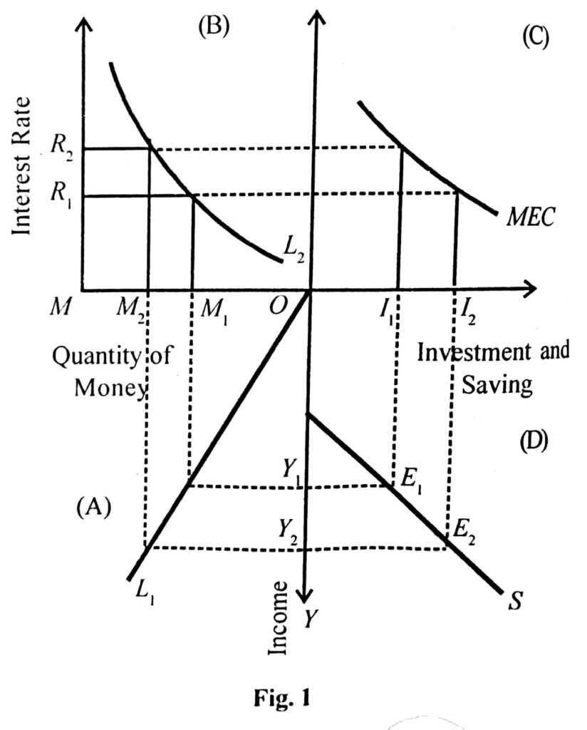
1. Thus at the OY1 income level, the transaction demand is given by OM1 and at the OY2 level of income, it is OM2. In Panel (B), the L2 curve represents the speculative demand for money as a function of the rate of interest.
2. When the rate of interest is R2, the speculative demand for money is MM2. With the fall in the rate of interest to R1, the speculative demand for money increases to MM1. Panel (C) shows investment as a function of the rate of interest and the MEC. Given the MEC, when the rate of interest is R2, the level of investment is OI1. But when the rate of interest falls to R1, investment increases to OI2.
3. “In the Keynesian analysis, the equilibrium level of employment and income is determined at the point of equality between saving and investment. Saving is a function of income, i.e. S=f (Y). It is defined as the excess of income over consumption, S=Y-C and income are equal to consumption plus investment.
4. Thus Y = C + I   Or Y-C = I,   Y-C = S   so I = S
5. So the equilibrium level of income is established where saving equals investment. This is shown in Panel (D) of Figure 1 where the horizontal axis from O toward the right represents investment and saving, and the OY axis represents income. S is the saving curve.
6. The line I1E1 is the investment curve (imagine that it can be extended beyond E as in an S and I diagram) which touches the S curve at E1. Thus OY1 is the equilibrium level of employment and income. This is the level of underemployment equilibrium, according to Keynes. If OY2 is assumed to be the full employment level of income then the equality between saving and investment will take place at E2 where I2E2 investment equals Y2E2 saving.

The Keynesian Theory of Income and Employment is also explained in terms of the equality of aggregate supply (C+S) and aggregate demand (C+I). Since unemployment results from the deficiency of aggregate demand, employment and income can be increased by increasing aggregate demand.

Assuming the propensity to consume to be stable during the short-run, aggregate demand can be increased by increasing investment. Once investment increases, employment, and income increase. Increased income leads to a rise in the demand for consumption goods which leads to a further increase in employment and income.

According to Keynes, the equilibrium level of employment will be one of under-employment equilibrium because when income increases consumption also increases but by less than the increase in income.

The Keynesian cross model of under-employment equilibrium is explained in Figure 2 where income and employment are taken on the horizontal axis and consumption and investment on the vertical axis. Autonomous investment is taken as a first approximation. C+I is the aggregate demand curve plotted by adding to consumption function C an equal amount of investment at all levels of income.

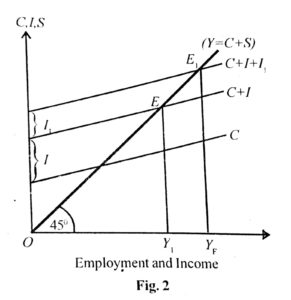The 45° line is the aggregate supply curve. The economy is in equilibrium at point E where the aggregate demand curves C+I intersects the 45° line. This is the point of effective demand where the equilibrium level of income and employment OY1 is determined.

1. This is the level of under­employment equilibrium and not of full employment. There are no automatic forces that can make the two curves cross at a full employment income level. If it happens to be a full-employment level, it will be accidental. Keynes regarded the under-employment equilibrium level as a normal case and the full employment income level as a special case.
2. Suppose OYF is the full employment income level. To reach this level, autonomous investment is increased by I1 so that the C+I curve shifts upward as C+I+I1, curve. This is the new aggregate demand curve that intersects the 45° line (the aggregate supply curve) at E1, the higher point of effective demand corresponding to the full employment income level OYF.
3. This also reveals that to get the desired increase in employment and income of Y1YF, it is the multiplier effect of an increase in investment by I1 (=I2 in Panel C of Figure 1) which leads to an increase in employment and income by Y1YF through successive rounds of investment.

For More Business Economic Notes Click Here

Credit reference: ML JINGAN 13th edition and The Keynesian Theory of Income, Output and Employment (yourarticlelibrary.com)