IS LM Model: General equilibrium of product and money Market

IS LM Model

• The IS-LM model explains by J M Keynes in the 1930s. The model was developed by the economist John Hicks in 1937 after Keynes published his book “The General Theory of Employment, Interest, and Money” in 1936.
• The IS-LM model, which stands for “investment savings” (IS) and “Liquidity preference-Money supply”

Goods Market Equilibrium – IS Curve

• IS curve is the combination of interest rates and investment where the goods market is in equilibrium
• The IS curve describes the goods market. The IS curve slopes down to the right, representing that as interest rates fall, people and businesses try to invest more in long-lasting goods like houses, cars, and equipment. When interest rates fall, families also tend to put less away for savings and spend more on consumer goods. Thus the effect of a falling interest rate is an increase in GDP through greater investment and less personal savings.
• The derivation of the IS curve is shown in Figures (A) and (B) The saving curve shows that saving increases as income increases, which means saving is an increasing function of income. On the other hand, Investment depends on the rate of interest and the level of income.

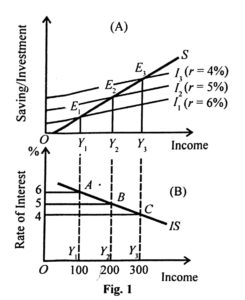
• In figure (A) At a 5% rate of interest, the investment curve is l₂. If the rate of interest is reduced to 4%, the investment curve will shift upward to l₃. The rate of investment will have to be raised to reduce the marginal efficiency of capital to equality with a lower rate of interest. Thus the investment curve shows more investment at every level of income.
• Similarly, when the rate of interest is raised to 6%, the investment curve will shift downward to l_1. The reduction in the rate of investment is essential to raise the marginal efficiency of capital to equality with a higher interest rate.
• In figure (B) IS curve shows the level of income at various interest rates. Each point on this IS curve represents a level of income at which saving equals investment at various interest rates.
• The rate of interest is represented on the vertical axis and the level of income on the horizontal axis. If the rate of interest is 6%, the S curve intersects the l₁  curve at E₁ which determines OY1 income. Similarly, when the rating of interest is from 5% to 4%, the S curve intersects to l2 and l3  curve at E2 to E3  which determines OY2 and OY3  income.
• By connecting these points to A, B, and C with a line, we get the IS curve. This IS curve slopes downward from left to right because as the interest rate falls, investment increases and so does income.
• In other words, there is a negative relationship between income and interest rate in the real sector of the economy. 

The Slop of the IS Curve

• Figure 1 (B) shows that the IS curve slope downward from left to right. This is a negative slope that reflects the increase in investment and income as the rate of interest falls.
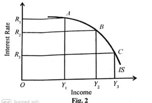
• If Investment is very sensitive to the rate of interest the Is curve is very flat. This is known as segment AB in figure 2 where small changes in the rate of interest lead to a change in the level of income.
• If the investment is not very sensitive to the rate of interest, the IS curve is relatively steep.

Shifts in the IS curve

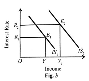
1. The IS function shifts to the right with a reduction in saving. A reduction in saving may be the result of one or more factors leading to increasing consumption. Consumers may like to buy the new products even by reducing savings.
2. The IS function also shifts to the right by an autonomous increase in investment. The increase in investment may result from expectations of higher profits in the future, from innovation, or expectations concerning the increase in the future demand for the product.  Moreover, governments’ expenditure and tax policies have the effects of shifting the IS function.

The Money Market Equilibrium (LM)

• The Money Market is in equilibrium when the demand and supply of money are equal. L stand for Money demand S stands for Money Supply, and in equilibrium L=M. The demand for money L=L_T+L_S where L_T is the transaction demand for money which is a direct function of the level of income. L_T =f(Y). L_S is speculative demand for money which is a decreasing function of the rate of interest, L_S = f(r). Thus money market equilibrium, M= L_T =f(Y) + L_S = f(r).

Deriving the LM Curve

The LM curve shows all combinations of interest rates and levels of income at which the demand for money and supply of money is equal. In other words, the LM curve shows the combinations of interest rates and levels of income where the demand for money (L) and supply of money (M) are equal such that the money market is in equilibrium.

The LM curve can be derived from the Keynesian formulation of liquidity preference.

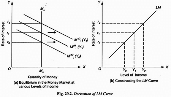
In Fig. 20.2 (b) we measure income on the X-axis and plot the income level corresponding to the various interest rates determined at those income levels through money market equilibrium by the equality of demand for and the supply of money in Fig. 20.2 (a).

The slope of the LM Curve:

• The above Fig. 20.2 (b) shows that the LM curve slopes upward to the right. This is because, with higher levels of income, the demand curve for money (Md) is higher and consequently the money-market equilibrium, the equality of the given money supply with the money demand curve occurs at a higher rate of interest. This implies that the rate of interest varies directly with income.
• It is important to know the factors on which the slope of the LM curve depends. There are two factors on which the slope of the LM curve depends. The first is the responsiveness of demand for money (i.e., liquidity preference) to the changes in income. As the income increases, say from Y0 to Y1, the demand curve for money shifts from Md0 to Md1, i.e., with an increase in income, demand for money would increase for being held for transactions motive, Md or L1 =f(Y).
• The second factor which determines the slope of the LM curve is the elasticity or responsiveness of demand for money (i.e., liquidity preference for a speculative motive) to the changes in the rate of interest. The lower the elasticity of liquidity preference for the speculative motive concerning the changes in the rate of interest, the steeper will be the LM curve. On the other hand, if the elasticity of liquidity preference (money demand function) to the changes in the rate of interest is high, the LM curve will be flatter or less steep.

Shifts in the LM Curve:

• The LM function shifts to the right with an increase in the money supply given the demand for money or due to the decrease in the demand for money on the given supply of money. If the central bank follows an expansionary monetary policy, it will buy securities in the open market. As a result, the money supply with the public increases for both transactions and speculative motives. This shifts the LM curve to the right.
• A decrease in the demand for money means a reduction in the number of balances demanded at each level of income and interest rate, which creates an excess of the money supply over the money demanded. This is equivalent to an increase in money supply in the economy which has the effect of shifting the LM curve to the right.
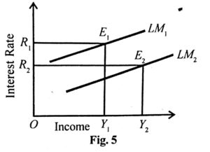
• Fig. 5 shows an increase in the money supply the LM₁ curve shifts to the right as LM₂ which moves the economy to a new equilibrium point E_2. The increase in the money supply brings down the rate to R₂ in the market.
• This in turn increases investment thereby the level of income to Y₂. Thus the effect of the increase in money supply is to shift the LM curve to the right and a new equilibrium is established at the lower interest rate, R_2, and higher income level, Y_2.  

The Money Market equilibrium

• Equilibrium in the economy occurs when both the money market and the product market are simultaneously in equilibrium.
• These two large markets interact, and the adjustments that occur in either of the markets will induce adjustments in the other market.

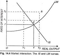
• The IS curve represents the relationship between the level of real output and the real interest rate, which generates equilibrium in the money market. These curves, for given levels of government expenditure, taxation, net exports, prices, and anticipated rate of price change are shown in Figure 14.4. Any changes in the conditions that are assumed given for these two curves would be shown as shifts in either the IS or the LM curve.
• Suppose that the economy was initially at a real interest rate of r2 and a level of real output of Y2. This is shown by the position in Figure 14.4. At a, both the product market and the money market are out of equilibrium. For the real interest rate of r2, there is not sufficient aggregate demand for real output to sustain the real income level of Y2
• Equilibrium in the product market for a real interest rate of r2 would occur at the level of real output Y1. At this point, aggregate demand is deficient. The unintended inventory accumulation will induce producers to cut back on their production. As a result, real income and employment will decline.
• Similarly, at the real income level of Y2, the real interest rate of r2 is too high for equilibrium in the money market. At this point, there is an excess supply of real money balances. Credit conditions will change as individuals attempt to remove these excess holdings of real money balances by acquiring additional bonds, and the market real rate of interest will decline.
• Both markets will continue to adjust until simultaneous equilibrium is reached. This equilibrium position for both the product and money markets is given by the intersection E of the IS LM model curves at the real income level Y with the real interest rate r.

For More Business Economic Notes Click Here

Reference: ML Jhingan, Economics Discussion, Manan Prakashan,yourarticlelibrary.com