Supply Analysis | Economics Class 12 Maharashtra Board

Supply Analysis

Economics 12th Standard HSC Maharashtra State Board Chapter – 4 Supply Analysis |Maharashtra State Board Class 12 Economics Solutions Chapter 4 Supply Analysis

Concept of Total Output, Stock, and Supply:

Total Output :

1. Output produced through the process of production. Input – processing – output
2. Output in economic is the “total quantity of goods or services produced in a given period of time by a firm, industry, or country”
3. Therefore, Total output is the total amount of commodities produced during a period of time with help of all factors of production employed by the firms.
   

   ---

Stock:

1. Stock is the total quantity of commodities available for sale with a seller at a particular point in time. Stock refers to the quantity possessed by a seller.
2. By increasing production, stock can be increased. Without stock, supply is not possible.
3. Normally, Stock can exceed supply and it is fixed and inelastic.
   In the case of perishable goods such as milk, fish, etc. stock may be equal to supply. On the other hand, durable goods such as furniture, garments, etc. stock can exceed the supply.

   ---

Supply:

1. The term ‘supply’ refers to the quantity of a commodity which the seller is willing and able to sell in the market at a particular price, during a given period of time.
2. According to Paul Samuelson, supply refers to “The relation between market prices and the number of goods that producers are willing to supply.”
3. Supply is a relative term. It is always expressed in relation to price, time, and quantity.
   

   ---

Individual Supply Schedule :

Individual supply refers to the various quantity of commodities, offered for sale by an individual seller/producer at different prices during a given period of time.

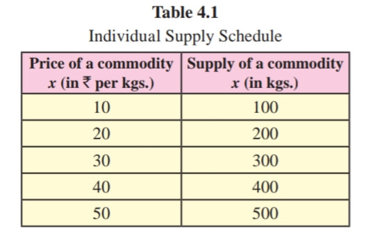
• Table 4.1 explains the functional relationship between price and quantity supplied of a commodity. Lower the price, lower the quantity of a commodity supplied, and vice versa.
• At the lowest price of ₹10, supply is also lowest at 100 kgs. At the highest price of ₹50, the quantity supplied is highest at 500 kgs.

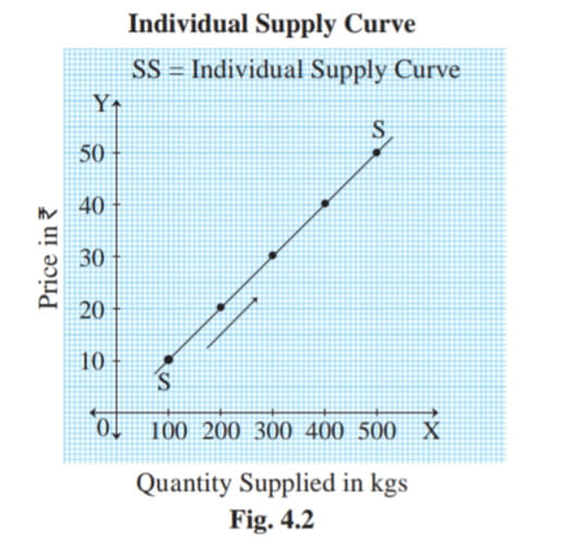
In figure 4.2, the quantity supplied is shown on the X-axis and the price on the Y-axis. Supply curve SS slopes upwards from left to right, indicating a direct relationship between price and quantity supplied.

Market supply

Market supply refers to the various quantity of commodities, offered for sale by all the sellers/producers at different prices during a given period of time.

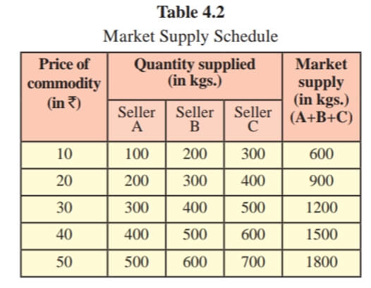
In Table 4.2, market supply is obtained by adding the supply of sellers A, B, and C at different prices. At the highest price of ₹ 50, market supply is the highest at 1800 kgs. At the lowest price of 10 market supply is the lowest at 600 kgs.

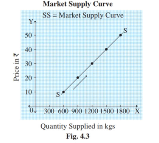
In figure 4.3, the quantity supplied is shown on the X-axis and the price on the Y-axis. Supply curve SS slopes upwards from left to right, indicating a direct relationship between price and market supply.

Determinants of supply factors determining supply

1. Price of a Commodity:– The supply of commodities is directly related to its price. Generally, more quantity of a commodity is offered for sale at a higher price, and less quantity is offered for sale at a lower price.
2. State of technology: – Technological improvements help not only improves the quality, but also the quantity of production. The quantity of production is increased due to the speed of the machines, and also there is a reduction in wastage. The increase in production facilities more supply in the market.
3. Cost of production: – If the cost of production rises i.e. if sellers have to pay more factors like rent, wages, interest, etc. thus, supply will be reduced.
4. Infrastructure facility: – Infrastructure in a form of transport, communication, etc. influences the production process and also supplies. And the shortage of these facilities decreases the supply.
5. Government policy: – Government policy affects the supply. For e.g., changes in taxation, industrial policies, sales tax, customs duties, etc. may encourage or discourage production and supply.
6. Natural conditions: – Natural factors like weather conditions, drought, floods, earthquakes, etc. can cause fluctuations in supply, especially in agricultural goods.
7. Future Expectation about price: – Expectations about the future price will affect the supply. If the price is expected to rise in the near future, the producer may hold on to the stock. This will reduce supply.
8. Exports and imports: – Export reduces the number of goods supplied within the country. Imports increase the supply in the domestic market.
9. Size of the market: – The size of the market greatly influences the supply. The larger the size of the market, there will more production and the larger will be the supply.
10. Nature of market: – Supply is influenced by the nature of the market. In a competitive market, the supply of goods would be more due to a large number of sellers. But in monopoly, i.e., single seller market, supply would be less.
11. Number of producers: – If there is a large number of producers, there will be large-scale production of a commodity, which leads to higher supply in the market. However, if the number of producers is very low, the production may be low and supply also would be low.
    

    ---

What is the Law of Supply?

Introduction:-

The law of supply is introduced by Dr. Alfred Marshall in his book ‘Principles of Economics,’ which was published in 1890. The Law of Supply explains the functional relationship between the price of the commodity and the quantity supplied in the market.

Statement of the Law:-

According to Dr. Alfred Marshall, “other thing being equal, higher the price of the commodity, greater is the quantity supplied and lowers the price of the commodity, smaller is the quantity supplied.”

More quantity of a commodity is offered for sale at a higher price and less quantity is offered for sale at lower prices. So the supply of a commodity is directly related to its price.

Sx = f (Px)

S = Supply,  x = Commodity f = Function,  P = Price of commodity

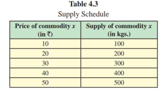
• Table 4.3 explains the direct relationship between the price and quantity of commodities supplied. When the price rises from ₹10 to 20, 30, 40, and 50, the supply also rises from 100 to 200, 300, 400, and 500 units respectively.
• It means, when price rises supply also rises and when the price falls supply also falls. Thus, there is a direct relationship between price and quantity supplied which is shown in following figure 4.4 :

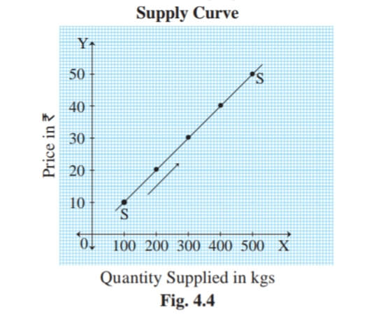
• In figure 4.4, X-axis represents the quantity supplied and Y-axis represents the price of the commodity. Supply curve ‘SS’ slopes upwards from left to right which has a positive slope.
• It indicates a direct relationship between price and quantity supplied.
  

  ---

 Assumptions of the law :

1. Constant cost of production: It is assumed that there is no change in the cost of production. If there is a change in the cost of production, it may affect the price of the commodity and its supply.
2. The constant technique of production: It is assumed that there is no change in the method or technique of production. Improvement in technology can increase the supply at the same price.
3. No change in weather conditions: It is assumed that there is no change in weather conditions. There are no natural calamities like floods, earthquakes which may decrease supply.
4. No change in Government policy: It is also assumed that government policies like taxation policy, trade policy, etc. remain unchanged.
5. No change in transport cost: – It is assumed that the transport cost remains unchanged. If a change in transport cost it affect the price of the commodity and their supply.
6. Price of other goods remains constant: – The prices of other goods are assumed to remain constant. If the price of other goods changes, then, the law of supply will not apply.
7. No future expectations: The law also assumes that the sellers do not expect future changes in the price of the product.
   

   ---

Exceptions to the Law of Supply :

Supply of labour: Labour supply is the total number of hours that workers work at a given wage rate. It is represented graphically by a supply curve. In the case of labour, as the wage rate rises the supply of labour (hours of work) would increase. So the supply curve slopes upward. Supply of labour (hours of work) falls with a further rise in wage rate and the supply curve of labour bends backward. This is because the worker would prefer leisure to work after receiving a higher amount of wages. Thus, after a certain point when the wage rate rises the supply of labour tends to fall.

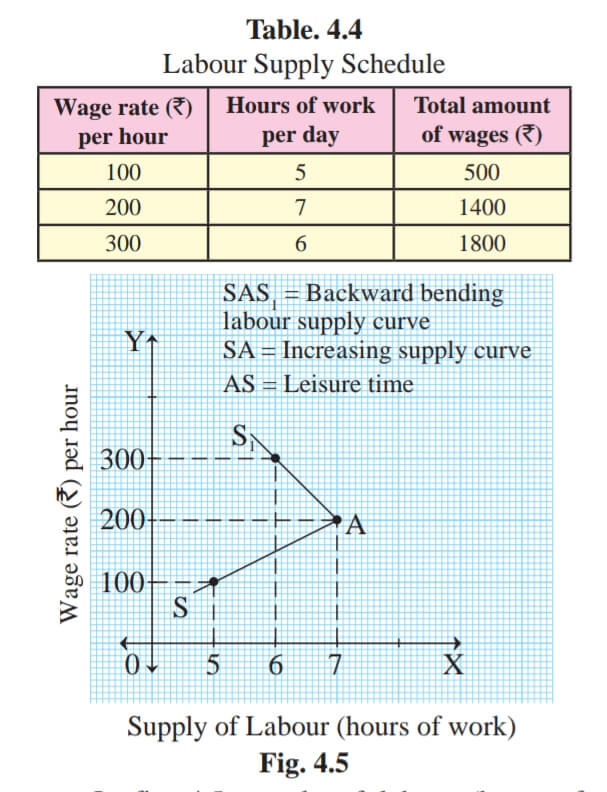
• It can be explained with the help of a backward bending supply curve. Table no. 4.4 and fig. no 4.5 explain the backward bending supply curve of labour.
• In fig. 4.5, the supply of labour (hours of work) is shown on X-axis, and the wage rate per hour is shown on the Y-axis. The curve SAS represents the backward bending supply curve of labour.
• Initially, when the wage rate is 100 per hour, the hours of work are 5. The total amount of wages received is 500. When the wage rate rises from 100 to 200, hours of work will also rise from 5 hours to 7 hours and the total amount of wages would also rise from 500 to 1400. At this point, labourer enjoys the highest amount
  i.e. 1400 and works for 7 hours.
• If the wage rate rises further from 200 to 300, the total amount of wages may rise, but the labourer will prefer leisure time and denies working for extra hours. Thus, he is ready to work only for 6 hours. At point A, the supply curve bends backward, which becomes an exception to the law of supply.

Agricultural goods: The law of supply does not apply to agricultural goods as they are produced in a specific season and their production depends on weather conditions. Due to unfavourable changes in weather, if agricultural production is low, their supply cannot be increased even at a higher price.

Urgent need for cash: – A businessman may face an urgent need for funds, and as such he may sell out more goods even at a lower price. This is an expectation of the law of supply.

Perishable goods:- The seller has to dispose of perishable goods like meat, fish, fruits, flowers, etc., even if the price falls. They cannot wait for a longer time for the price to rise, in order to increase supply.

Rare goods: The supply of rare goods cannot be increased or decreased according to their demand. Even if the price rises, supply remains unchanged. For example, rare paintings, old coins, antique goods, etc.

Variations in Supply :

When quantity supplied of a commodity varies due to change in its price, other factors remaining constant, it is known as variations in supply. There are two types of variations in supply :

Expansion of supply :

Expansion of supply refers to a rise in the quantity supplied due to a rise in the price of a commodity, other factors remaining constant. Expansion in supply leads to an upward movement on the same supply curve due to a rise in price. It is shown in figure 4.6

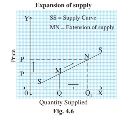
In figure 4.6, the quantity supplied is shown on the X-axis and the price on the Y-axis. Quantity supplied rises from OQ to OQ1, with a rise in price from OP to OP1, resulting in an upward movement from M to N along the same supply curve SS. It is known as the Expansion of supply.

Contraction of supply :

Contraction of supply refers to a fall in the quantity supplied, due to a fall in the price of a commodity, other factors remaining constant. In the case of contraction of supply, there is a downward movement on the same supply curve. It is shown in figure 4.7

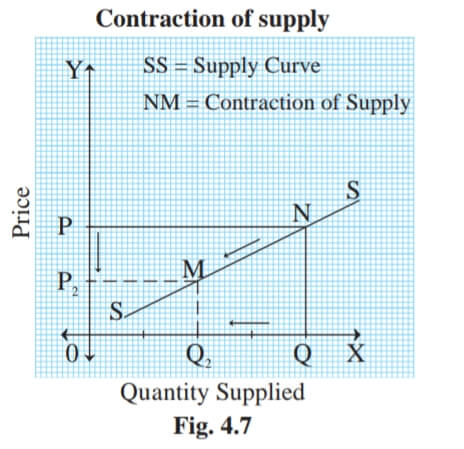
In figure 4.7, the quantity supplied is shown on the X-axis and the price on the Y-axis. Quantity supplied falls from OQ to OQ2 with a fall in price from OP to OP2, resulting in a downward movement from N to M on the same supply curve SS. It is known as Contraction of supply.

Changes in Supply :

When other factors change and price remains constant, it is known as changes in supply. There are two types of changes in supply :

Increase in supply :

An increase in supply refers to a rise in the supply of a given commodity due to favourable changes in other factors such as a fall in the price of inputs, a fall in tax rates, technological up-gradation, etc., while price remains constant. The supply curve shifts to the right of the original supply curve. It is shown in figure 4.8

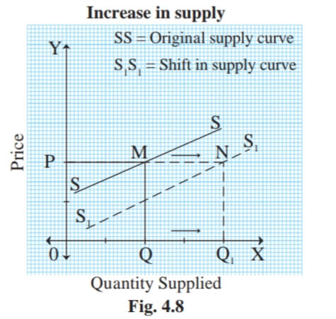
In figure 4.8, the quantity supplied is shown on the X-axis and the price on the Y-axis. Supply rises from OQ to OQ1 at the same price OP, resulting in an outward shift of the original supply curve to the right from SS to S1S1. It is known as an increase in supply.

Decrease in supply :

A decrease in supply refers to a fall in the supply of a given commodity due to unfavourable changes in other factors such as an increase in the prices of inputs, an increase in the tax rate, outdated technology, strikes by workers, and the price remains constant. The supply curve shifts to the left of the original supply curve. It is shown in figure 4.9

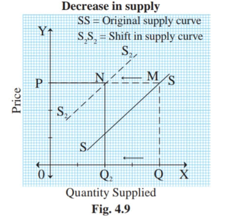
In figure 4.9, the quantity supplied is shown on the X-axis and the price on the Y-axis. Supply falls from OQ to OQ2 at the same price OP, resulting in an inward shift of the original supply curve to the left from SS to S2S2. It is known as a Decrease in supply.

Concepts of Cost and Revenue:

Total Cost (TC):

Total cost is the total expenditure incurred by a firm on the factors of production required for the production of goods and services. Total cost is the sum of total fixed cost and total variable cost at various levels of

TC = TFC + TVC

TC = Total cost

TFC = Total Fixed Cost

TVC = Total Variable Cost

Total Fixed Cost (TFC): Total fixed costs are those expenses of production which are incurred on fixed factors such as land, machinery, etc.
Total Variable Cost (TVC): Total variable costs are those expenses of production which are incurred on variable factors such as labour, raw material, power, fuel, etc.

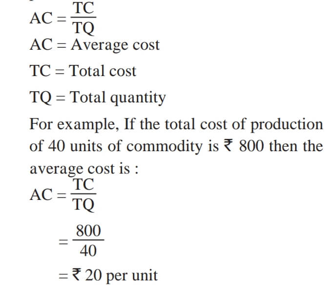
Average Cost (AC):

The average cost refers to the cost of production per unit. It is calculated by dividing total cost by total quantity of production.

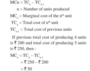
Marginal cost (MC):

Marginal cost is the net addition made to total cost by producing one more unit of output.

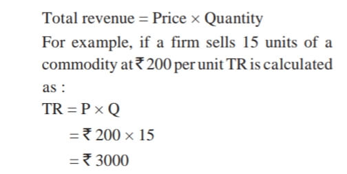
Total Revenue (TR):

Total revenue is the total sales proceeds of a firm by selling a commodity at a given price. It is the total income of a firm. Total revenue is calculated as follows :

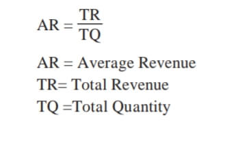
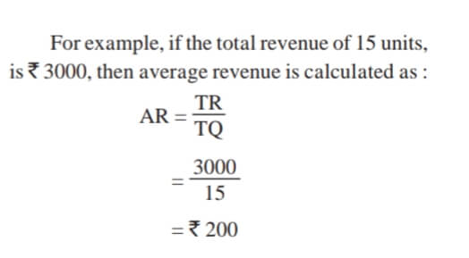
Average Revenue (AR):

Average revenue is the revenue per unit of output sold. It is obtained by dividing the total revenue by the number of units sold.

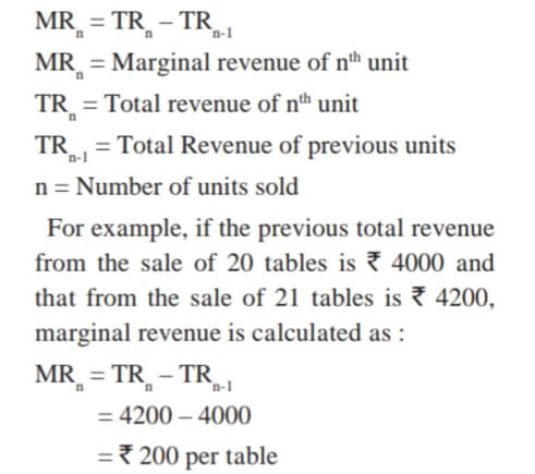
Marginal Revenue:

Marginal revenue is the net addition made to total revenue by selling an extra unit of the commodity.

Important Question of Economics Click Here 

Download PDF Board Sample  Paper with Solution – Click Here

For Other Subjects Click Here

Reference: MHSB books

This article includes: supply analysis, supply analysis notes, the law of supply with assumption and exception, economics class 12 maharashtra board pdf, Economics 12th, Maharashtra State Board Class 12 Economics Solutions, types of variation in supply, difference between variation in supply and changes in supply, 12th commerce economics textbook solutions 2021, economics class 12 maharashtra board pdf, sc class 12 economics chapter wise notes.